State estimation
It is often easy enough to write down equations determining the dynamics of a system: how its state varies over time. Given a system at time k we can predict what state it will be in at time k+1. We can also take measurements on the system at time k+1. The process of fusing zero or measurements of a system with predictions of its state is called state estimation.
The Kalman filter
A very popular state estimation algorithm is the Kalman filter. The Kalman filter can be used when the dynamics of a system are linear and measurements are some linear function of state.
Problem formulation
Let’s first refresh the goal of the Kalman filter and its formulation. The Kalman filter attempts to update an estimate of the “true” state of a system given noisy measurements of the state. The state is assumed to evolve in a linear way and measurements are assumed to be linear functions of the state. Specifically, it is assumed that the “true” state at time \(k+1\) is a function of the “true” state at time \(k\):
where \(w_k\) is a sample from a zero-mean Gaussian process with covariance \(Q_k\). We term \(Q_k\) the process covariance. The matrix \(F_k\) is termed the state-transition matrix and determines how the state evolves. The matrix \(B_k\) is the control matrix and determines the contribution to the state of the control input, \(u_k\).
At time instant \(k\) we may have zero or more measurements of the state. Each measurement, \(z_k\) is assumed to be a linear function of the state:
where \(H_k\) is termed the measurement matrix and \(v_k\) is a sample from a zero-mean Gaussian process with covariance \(R_k\). We term \(R_k\) the measurement covariance.
The Kalman filter maintains for time instant, \(k\), an a priori estimate of state, \(\hat{x}_{k|k-1}\) covariance of this estimate, \(P_{k|k-1}\). The initial values of these parameters are given when the Kalman filter is created. The filter also maintains an a posteriori estimate of state, \(\hat{x}_{k|k}\), and covariance, \(P_{k|k}\). This is updated for each measurement, \(z_k\).
Example: the constant velocity model
The Kalman filter is implemented in Starman in the
starman.KalmanFilter class. This section provides an example of use.
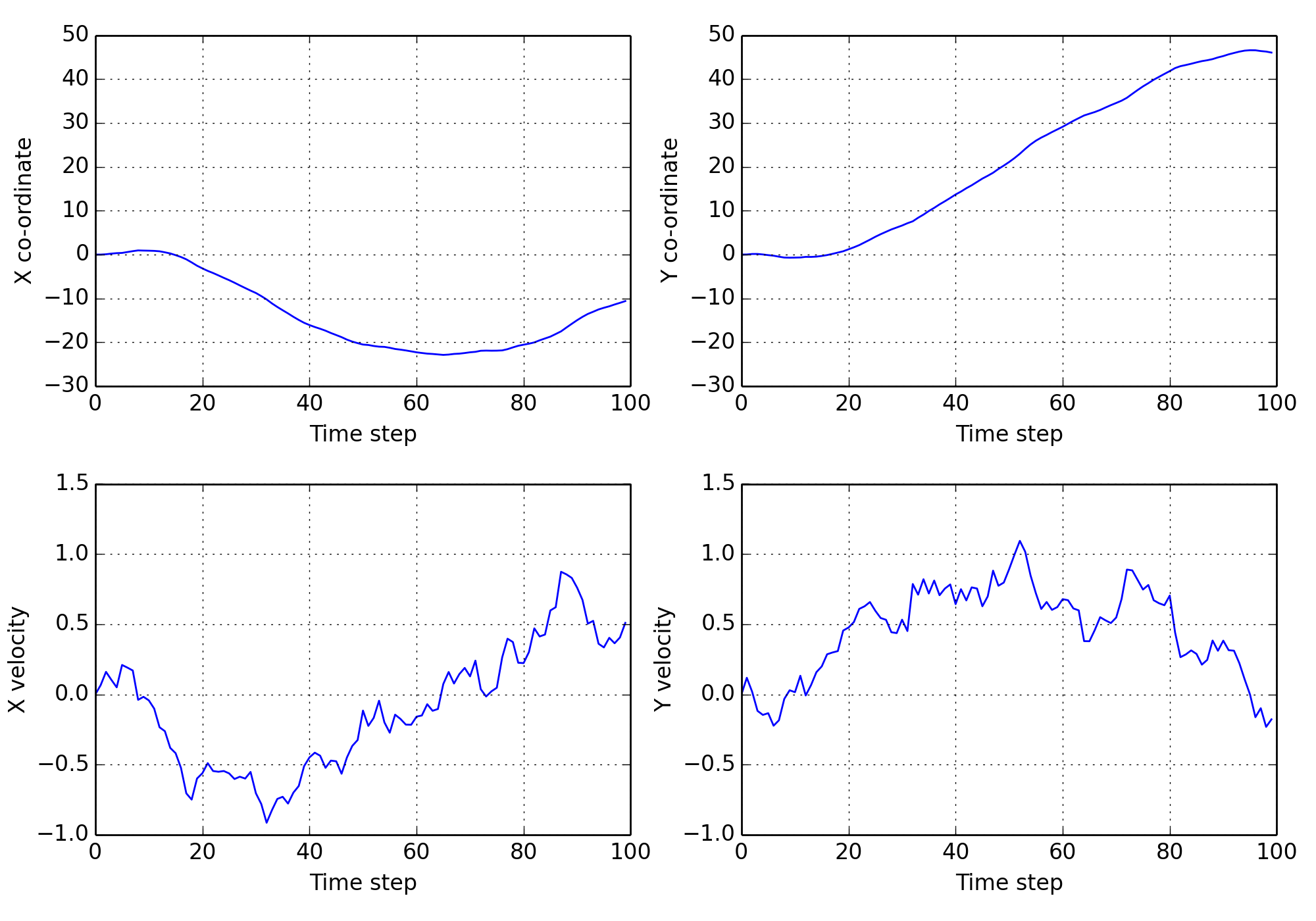
Generating the true states
We will implement a simple 2D state estimation problem using the constant velocity model. The state transition matrix is constant throughout the model:
# Import numpy and matplotlib functions into global namespace
from matplotlib.pylab import *

# Our state is x-position, y-position, x-velocity and y-velocity.
# The state evolves by adding the corresponding velocities to the
# x- and y-positions.
F = array([
    [1, 0, 1, 0], # x <- x + vx
    [0, 1, 0, 1], # y <- y + vy
    [0, 0, 1, 0], # vx is constant
    [0, 0, 0, 1], # vy is constant
])

# Specify the length of the state vector
STATE_DIM = F.shape[0]
Let’s generate some sample data by determining the process noise covariance:
# Specify the process noise covariance
Q = diag([1e-2, 1e-2, 1e-1, 1e-1]) ** 2

# How many states should we generate?
N = 100

# Generate some "true" states
from starman.linearsystem import generate_states
true_states = generate_states(N, process_matrix=F, process_covariance=Q)
assert true_states.shape == (N, STATE_DIM)
We can plot the true states we’ve just generated:
(Source code, png, hires.png, pdf)
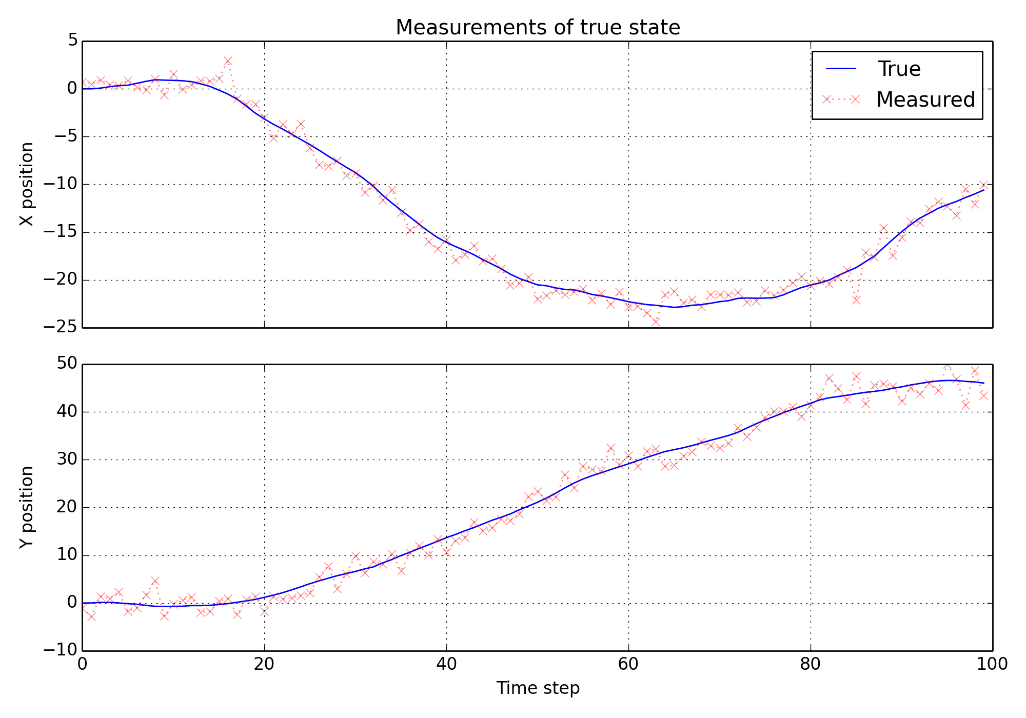
Generating measurements
We will use a measurement model where the velocity is a “hidden” state and we can only directly measure position. We’ll also specify a measurement error covariance.
# We only measure position
H = array([
    [1, 0, 0, 0],
    [0, 1, 0, 0],
])

# And we measure with some error. Note that we have difference
# variances for x and y.
R = diag([1.0, 2.0]) ** 2

# Specify the measurement vector length
MEAS_DIM = H.shape[0]
From the measurement matrix and measurement error we can generate noisy measurements from the true states.
# Measure the states
from starman.linearsystem import measure_states
measurements = measure_states(true_states, measurement_matrix=H,
                              measurement_covariance=R)
Let’s plot the measurements overlaid on the true states.
(Source code, png, hires.png, pdf)
Using the Kalman filter
We can create an instance of the starman.KalmanFilter to filter our
noisy measurements.
from starman import KalmanFilter, MultivariateNormal

# Create a kalman filter with constant process matrix and covariances.
kf = KalmanFilter(state_length=STATE_DIM,
                  process_matrix=F, process_covariance=Q)

# For each time step
for k, z in enumerate(measurements):
    # Predict state for this timestep
    kf.predict()

    # Update filter with measurement
    kf.update(measurement=MultivariateNormal(mean=z, cov=R),
              measurement_matrix=H)
The starman.KalmanFilter class has a number of attributes which
give useful information on the filter:
# Check that filter length is as expected
assert kf.state_count == N

# Check that the filter state dimension is as expected
assert kf.state_length == STATE_DIM
Now we’ve run the filter, we can see how it has performed. We also shade the three sigma regions for the estimates.
(Source code, png, hires.png, pdf)
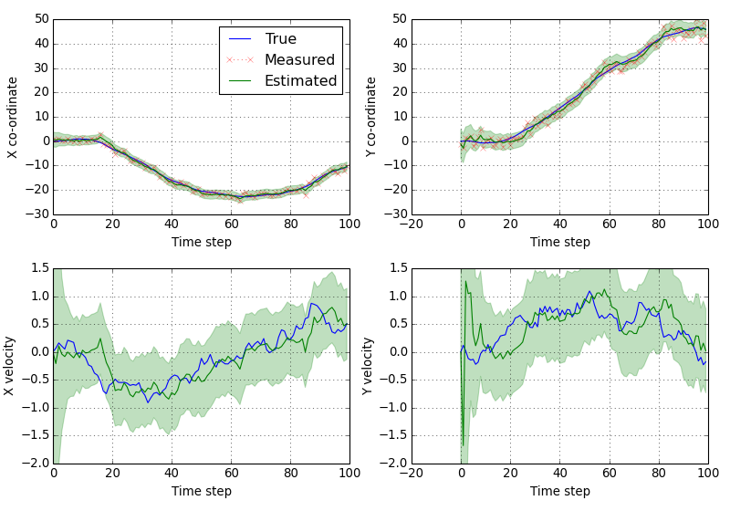
We see that the estimates of position and velocity improve over time.
Rauch-Tung-Striebel smoothing
The Rauch-Tung-Striebel (RTS) smoother provides a method of computing the “all data” a posteriori estimate of states (as opposed to the “all previous data” estimate). Assuming there are \(n\) time points in the filter, then the RTS computes the a posteriori state estimate at time \(k\) after all the data for \(n\) time steps are known, \(\hat{x}_{k|n}\), and corresponding covariance, \(P_{k|n}\), recursively:
with \(C_k = P_{k|k} F^T_{k+1} P_{k+1|k}^{-1}\).
The RTS smoother is an example of an “offline” algorithm in that the estimated state for time step \(k\) depends on having seen all of the measurements rather than just the measurements up until time \(k\).
Using RTS smoothing
We’ll start by assuming that the steps in Example: the constant velocity model have been
performed. Namely that we have some true states in true_states, measurements
in measurements and a starman.KalmanFilter instance in kf.
Following on from that example, we can use the starman.rts_smooth()
function to compute the smoothed state estimates given all of the data.
from starman import rts_smooth

# Compute the smoothed states given all of the data
rts_estimates = rts_smooth(kf)
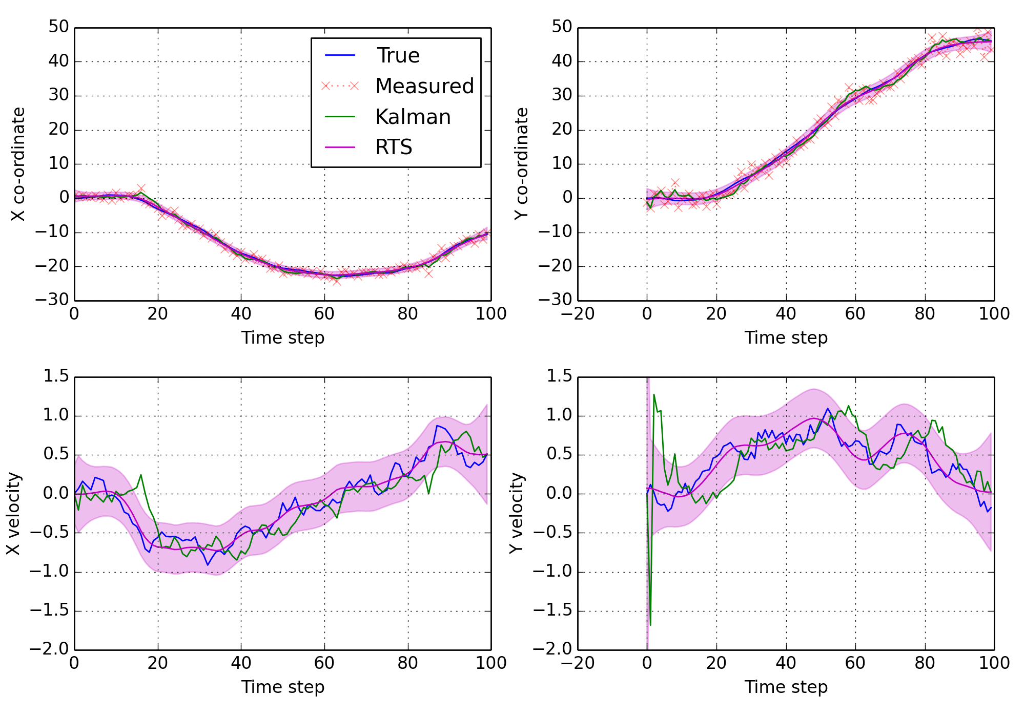
Again, we can plot the estimates and shade the three sigma region.
(Source code, png, hires.png, pdf)

We can see how the RTS smoothed states are far smoother than the forward estimated states. But that the true state values are still very likely to be within our three sigma band.
Mathematical overview
The Kalman filter alternates between a predict step for each time step and zero or more update steps. The predict step forms an a priori estimate of the state given the dynamics of the system and the update step refines an a posteriori estimate given the measurement.
A Priori Prediction
At time \(k\) we are given a state transition matrix, \(F_k\), and estimate of the process noise, \(Q_k\). Our a priori estimates are then given by:
Innovation
At time \(k\) we are given a matrix, \(H_k\), which specifies how a given measurement is derived from the state and some estimate of the measurement noise covariance, \(R_k\). We may now compute the innovation, \(y_k\), of the measurement from the predicted measurement and our expected innovation covariance, \(S_k\):
Update
We now update the state estimate with the measurement via the so-called Kalman gain, \(K_k\):
Merging is straightforward. Note that if we have no measurement, our a posteriori estimate reduces to the a priori one: