Feature Association
When estimating the state of a single system, techniques such as Kalman filtering can be extremely useful. Real situations often have several systems acting independently each of which can generate a measurement. Sometimes it is clear which measurement has arisen from which system. Sometimes it is not. Feature association is the process of associating actual measurements with predicted measurements from a set of tracked systems.
Scott and Longuet-Higgins association
The Scott and Longuet-Higgins algorithm [SLH] is an elegant algorithm for associating two sets of features by considering the Gaussian weighted distances between each pair of features. Since it considers pair-wise distances, and then uses an SVD, its computational complexity is approximately \(O(n^2)\).
In tracking problems we can use the SLH algorithm when we have good estimates of the predicted measurement estimate covariance and actual measurement covariance.
Example: 2D tracking
Let’s first of all create a list of “true” 2D locations of some set of targets. We’ll simply sample their location uniformly from the interval \((0, 10] \times (0, 10]\):
# Import plotting and numpy functions
from matplotlib.pylab import *

# How many targets?
n_targets = 25

# Sample the ground truth (gt) positions
gt_positions = 10 * np.random.rand(n_targets, 2)
We will simulate some tracking problem by assuming we’ve been tracking the targets and creating some estimates of state. We’ll let a certain proportion of the ground truth states be “new” states.
from numpy.random import multivariate_normal as sample_mvn
from starman import MultivariateNormal

def simulate_tracking_state(ground_truth):
    """Given a ground truth location, return a MultivariateNormal
    representing a simulated tracking state."""

    # Sample estimate covariance.
    cov = 1e-1 * np.diag(5e-1 + np.random.rand(2))
    cov[1, 0] = cov[0, 1] = 1e-1 * (np.random.rand() - 0.5)

    # Sample mean of estimate based on covariance
    mean = sample_mvn(mean=ground_truth, cov=cov)

    return MultivariateNormal(mean, cov)

# Sample our simulated state estimates. There's a probability of 0.1 that
# the ground truth state is a new one for this time step.
estimates = [simulate_tracking_state(s)
             for s in gt_positions if np.random.rand() < 0.9]
Now we’ll simulate measurements on the ground truth states. Again there is a proportion of states which we do not measure but each measurement has the same covariance.
from starman.linearsystem import measure_states

# Set measurement covariance
measurement_covariance = np.diag([1e-1, 1e-1]) ** 2

# Get list of MultivariateNormal instances for each measurement. We have
# a probability of 0.1 of missing a state.
gt_measurements = measure_states(gt_positions, np.eye(2),
                                 measurement_covariance)
measurements = [
    MultivariateNormal(mean=measurement, cov=measurement_covariance)
    for measurement in gt_measurements if np.random.rand() < 0.9
]
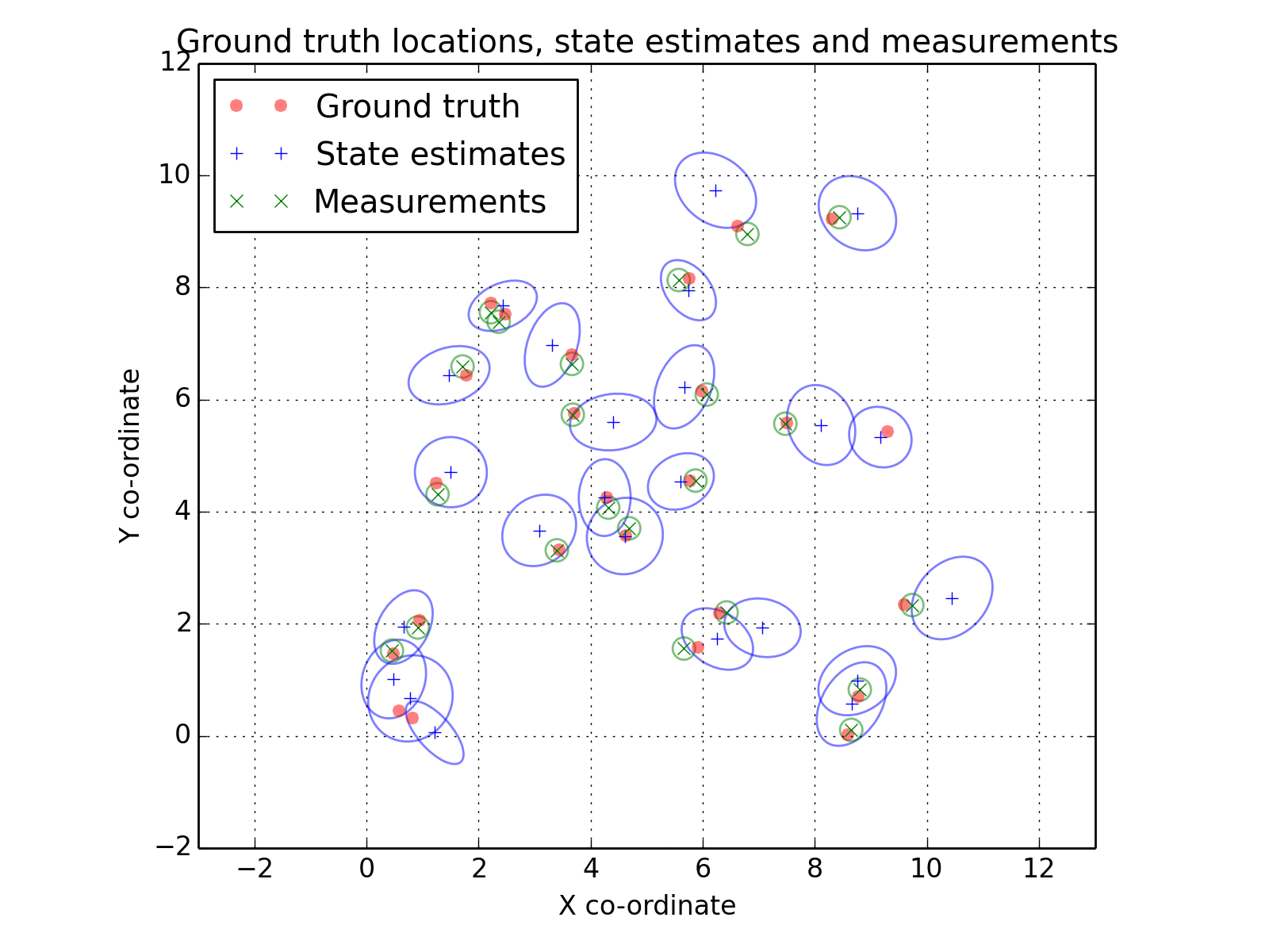
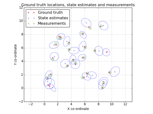
Let’s take a look at out ground truth positions and current tracking state estimates. We’ll plot a 2-sigma ellipse around each state estimate and each measurement.
(Source code, png, hires.png, pdf)
The SLH algorithm is implemented in the slh_associate() function. It
takes as non-optional arguments two lists of MultivariateNormal
instances which should be associated. It also takes an optional parameter
giving the maximum number of standard deviations two features can be separated
before they are considered to be impossible to associate. In this example we’ll
use the default 5-sigma separation threshold.
from starman import slh_associate

# Use slh_associate to associate state estimates with measurements.
associations = slh_associate(estimates, measurements)

# Associations are represented by an Nx2 array of indices into the two
# lists.
assert associations[:, 0].max() < len(estimates)
assert associations[:, 1].max() < len(measurements)
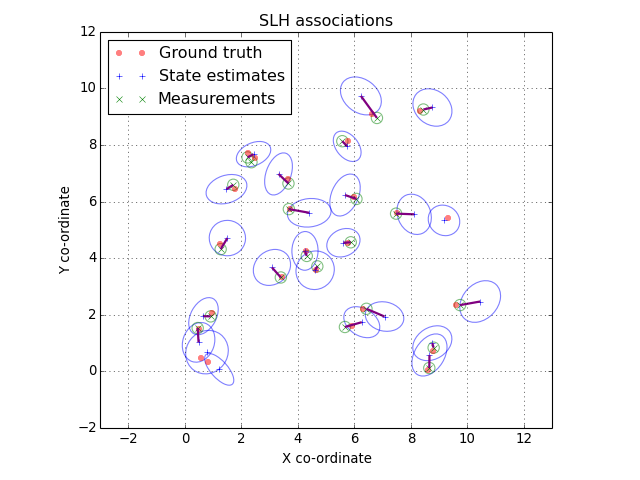
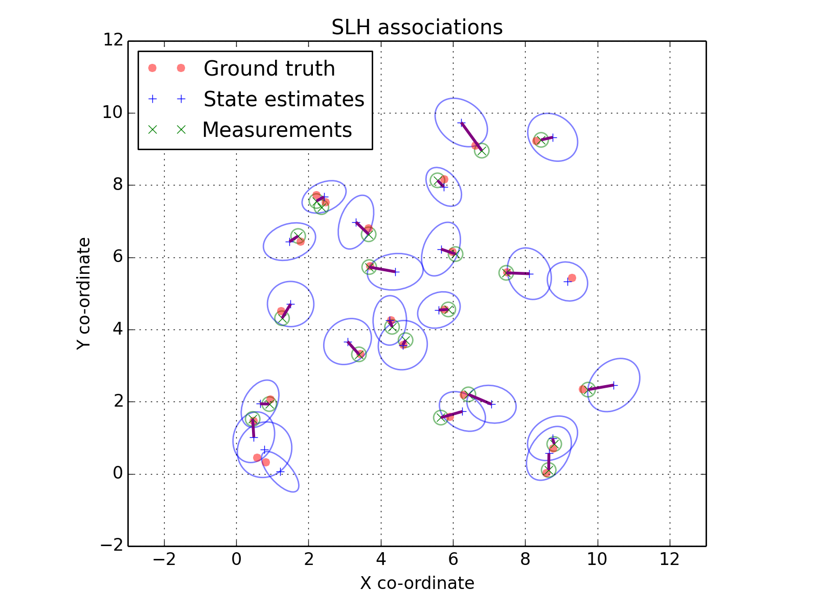
The associations are returned as a two-column array. The first column contains indices into the first list of features and the second column contains indices into the second list. For example we could turn the associations into a list of state estimate mean, measurement pairs:
associated_positions = []
for est_idx, meas_idx in associations:
    associated_positions.append([
        estimates[est_idx].mean, measurements[meas_idx].mean
    ])
(Source code, png, hires.png, pdf)

Mathematical overview
The SLH algorithm starts by assuming that there are two sets of features. Each feature is parametrised by a mean and covariance. We shall notate the \(i\)-th mean of group \(k\) as \(\mu_i^{(k)}\) and the \(i\)-th covariance of group \(k\) as \(\Sigma_i^{(k)}\). We then form a Gaussian weighted proximity matrix, \(G\), where
Our intution is that “true” associations are represented by a) a value close to 1 in \(G\) and b) that value being the largest in both its row and column. The “ideal” \(G\) is one where there is at most a single 1 in each row an column and every other element is zero. (This ideal matrix being orthogonal.) The SLH algorithm attempts to magnify the orthogonality of \(G\) by way of the singular value decomposition (SVD).
One firstly takes the SVD of \(G\) which finds \(U, S\) and \(V\) such that
The matrix of singular values \(S\) only has non-zero elements on its diagonal. Form a new matrix \(\Lambda\) from \(S\) by setting all non-zero elements to 1. Then form \(P\) as
Associate feature \(i\) in list 1 with feature \(j\) in list 2 if and only if:
- Element \(P_{ij}\) is the maximum in its row and column.
- \(G_{ij}\) is greater than some association threshold, \(\alpha\).
In practice the association threshold is set with reference to some number of standard deviations, \(\sigma\). So, \(\alpha = \exp(- \sigma^2 / 2)\).
The SLH algorithm can be interpreted as minimising the sum of squared distances between features where those distances are normalised by the covariance matrices of the features.
| [SLH] | Scott, Guy L., and H. Christopher Longuet-Higgins. “An algorithm for associating the features of two images.” Proceedings of the Royal Society of London B: Biological Sciences 244.1309 (1991): 21-26. |